The modulation transfer function (MTF) is a pretty commonly discussed concept in optics/physics fields, owing to its necessity in describing the consistency of optical configurations when acquiring images of features which can easily be convoluted. As I haven’t blogged for a bit I thought I’d do a longer piece on what MTF is, why it matters and how we might incorporate it into a UAV survey setup/use MTF charts to predict accuracy of mosaics/reconstructions in photogrammetry.
The Nyquist limit
When we take a photo, how will we know the difference between say, one shipping container and another? In this classic example, we can downsample this image of a bustling port to the point where the crates are indistuinguishable, ask questions about why this is happening, and how we might quantify it. The original image is shown below.
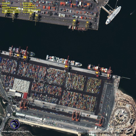
WORLDVIEW-2 FIRST IMAGE: PORT BOTANY, AUSTRALIA-OCTOBER 20, 2009: This image is a satellite image of Port Botany, Australia (credit:DigitalGlobe)
We can zoom in to part of it, and by downsampling we can try to generate an intuition of how different imaging resolutions will effect our ability to recover each individual crate.
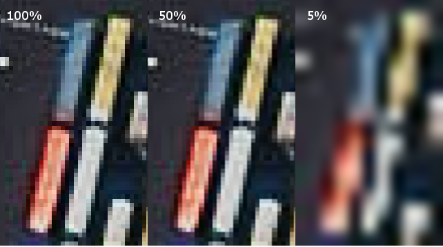
Original image downsampled and resized to give an artificially produced change in spatial (sampling) resolution
It seems like not much of a difference happens when we half the resolution for these particular features, but when we downsampled to a 20th of the resolution things become a little more interesting. To illustrate this more, we can run a canny filter, which is a very commonly used edge detection filter to try and automatically extract the crates’ edges.
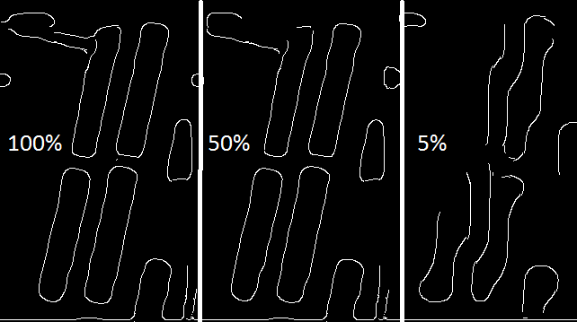
Canny filter of the image above
It looks like for an automatic crate detector with crates in this particular configuration downsampling to 5% of the original yields a result without much value. The edge detector (While we might optimize its parameters) can’t distinguish the edges of the crates, and neither can I by sight.
There’s a bunch of reasons why the practical limit exists for this particular image, but the principle of sampling resolution is the one I’d like to get at. How many pixels do you need to form an image? How many pixels do you need to identify a feature?
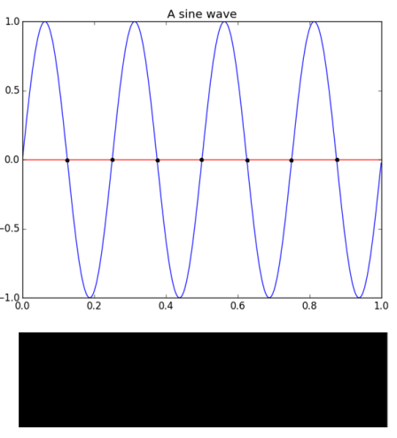
The Nyquist limit gives us the theoretical limit for this, and is well studied in the field of astronomy, which has a degree of overlap with photogrammetry. In order to recover the edge of a crate, such as in our example above, we must have at least one sample in the space between the them. A visualisation of what this looks like is presented below, with the peaks of the sin wave analogous to a crate being present, and edges of crates at x=0. If we sample at a rate less than this, we start to get artifacts (‘Aliasing’) and convolutions in the signal which means detection of individual bands will be ill-posed.
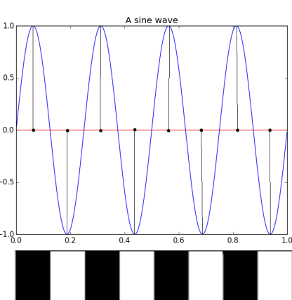
A sin wave sampled at the Nyquist frequency, with the image analogue below. In reality the image represents a square function
In the example of the sin wave, the signal is perfectly recoverable. Theoretically, in order to sample at a rate at or above the rate suggested by the Nyquist frequency, we should be sampling at the very least on the order of the size of the objects/waves for resolving to say whether they are different things. If we, for example sample our sin wave as before, but begin sampling half a wavelength across (‘Phase-shifted’), we get ‘aliasing’.
Aliased signal, undersampling leads to no signal being resolved
While the former image recovered the image perfectly, the latter could not reconstruct any of the sin wave, the ability of the imaging system not only to record accurately, but to choose a sensible sampling rate is what choice of resolution boils down to. As a rule of thumb, you generally need at least three pixels to tell if an object really exists in a image.
MTF
Armed with the basics of this idea, we can calculate the absolute minimum our resolution needs to be to resolve two objects, but MTF comes in to the physical side of things. Due to distortions present in ever lens system (Note: MTF is specific to each lense) and in sensor setup the conservation of contrast isn’t so simple. MTF can give us a quick idea of how a lens will perform based on the distance from the centre of the image, where not only will the real-world sampling rate decrease (off-nadir) but the quality of each pixel will degrade. The whole reason for briefly looking at Nyquist is that is exactly what MTF tells us; the ability of the lens to resolve bands of high contrast at different distances apart. Let’s have a look at an MTF chart,
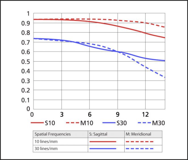
Sample MTF chart, taken from Nikon’s site here
So, the red lines show the lens’ ability to resolve lines located .1mm apart for lines running both parellel (‘Sagittal’) and perpendicular (‘Meridional’) from the centre to the edges of an image.
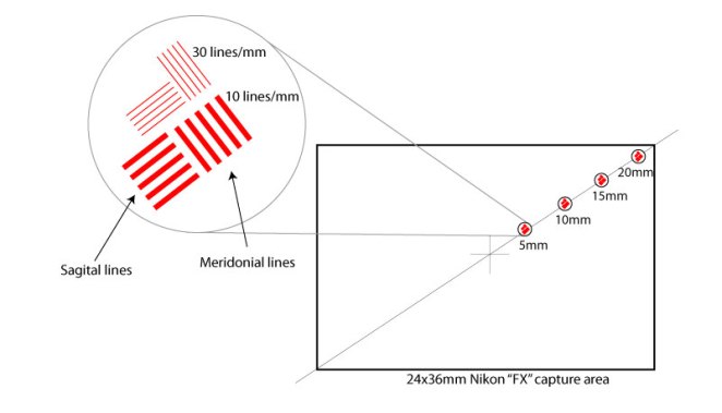
MTF tests ability to recover Sagittal and Meridonial lines
The blue lines do the same, but at a spacing of .033mm. The x axis shows distance in mm from the centre of the image, and the y axis shows the MTF index, or how accurately the lens can resolve the sets of lines. We can see the general trend that accuracy in resolution (acutance) reduces if we move away from the image centre for all sets of measurements. We see that MTF is lower for line pairs which are closer together, and that meridonial lines at 30mm apart show the worst performance at image edges.
Standard charts are made by the international organization for standardization, an example is given below for not only measuring MTF, but also colour contrasts and accuracy of resolving chequered targets, all of which are standard tasks within trying to undistort images/measure their quality.
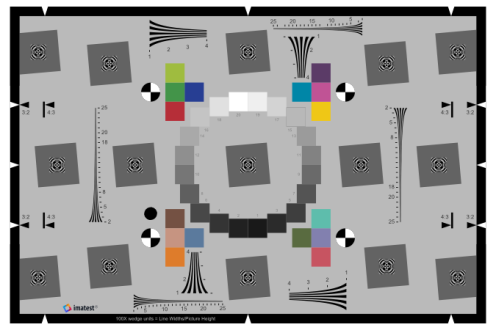
12233:2014 test chart for measuring MTF, taken from here
MTF will change with both aperture and focal length, and DxoLabs have some pretty neat graphics to illustrate this. As shown below, a lens’ ability to resolve is greater for bigger apertures (smaller f numbers) where diffraction is not an issue. Generally, shorter focal lengths show a better ability to resolve line pairs which are closer together (The metric used here), and longer focal lengths struggle as bigger apertures (small f numbers) due to increasing image softness.
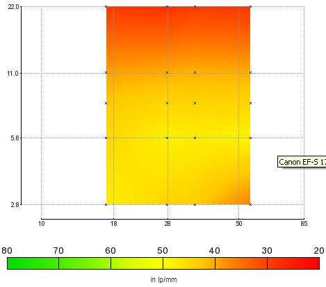
From DxOLabs page, here
Too much information?
MTF, Nyquist limits and diffraction, do we really need this depth of information for something as seemingly simple as taking a digital photo? What are the benefits of thinking this deeply about the equipment and the settings we use?
MTF gives us very easy to use, practical information about the lens, and when planning campaigns we can use this to predict how fine a level of detail we can resolve. Particularly for metric applications it will allow us to know ahead of time whether our survey will be sufficient for the task at hand.
For image matching, difference of gaussian operators operate on a sub-pixel level, and so any more accurate contrast preservation will benefit their localisation. In turn, this will effect the accuracy of the subsequent photogrammetric reconstructions.
Modelling the effect MTF has on metric outputs, combined with their impacts on building proper camera models is an important concept moving forward. With the increasing use of consumer cameras for SfM and photogrammetric applications, ensuring image quality must be a priority for anyone in the field.
